Impressed currents: driving a model with a known current

Not every drive is a port. Sometimes the current is the thing you know — a coil wound to a specification, an interference current measured on a harness, a lightning channel, a probe injecting a known signal — and what you want out of the simulation is the field it produces. SourceCurrentPath says exactly that: a current I(t) prescribed along a curve through the model.

This page calibrates the source against two textbook antennas, which is the useful thing to do once before trusting it on a real structure: a short filament in free space (the Hertzian dipole) and the same filament standing on a ground plane (the short monopole). Each gives a radiated power and a directivity that are known in closed form, so a single number per case says whether the current that reached the grid is the current that was asked for.

import matplotlib.pyplot as plt
import numpy as np

import magnelio as mio
from magnelio import geo, monitors, signals, sources
from magnelio.constants import C0, ETA0

F0 = 5e9  # the frequency the pattern is read at
F_MAX = 10e9  # the analysis band
HALF = 90e-3  # half the domain edge [m] — 1.5 λ of clearance at F0
LENGTH = 5e-3  # filament length [m], λ/12 at F0
OPEN = dict.fromkeys(("xmin", "xmax", "ymin", "ymax", "zmin", "zmax"), "CPML")


def air_box(boundaries, z0=-HALF, height=2 * HALF):
    model = mio.GeometryModel(boundary_conditions=boundaries)
    model.add(
        geo.Brick(origin=(-HALF, -HALF, z0), size=(2 * HALF, 2 * HALF, height), material="air")
    )
    return model


def radiate(model, name):
    """One transient run; returns the far-field pattern at ``F0``."""
    mesh = mio.Mesh.from_geometry(model, mio.MeshControl(min_nodes_per_wavelength=12), f_max=F_MAX)
    pattern = monitors.MonitorFarFieldFrequency(name="pattern", freqs=[F0], margin_cells=2)
    result = mio.AnalysisTD(mesh=mesh, monitors=[pattern], verbose=False).run(
        excitations=[
            mio.Excitation(name, waveform=signals.WaveformGaussian(f_max=F_MAX), amplitude=1.0)
        ],
        t_end=2000e-12,
        energy_stop_db=60,
    )
    result.renormalize(name)
    return pattern.result(F0)

A filament in free space

The path is a list of points — here just two, five millimetres apart — and the excitation carries the current in amperes. The endpoints become grid planes, so the filament is exactly as long as it was declared, whatever the cell size.

model = air_box(OPEN)
model.add_source(
    sources.SourceCurrentPath(name="fil", path=[(0, 0, -LENGTH / 2), (0, 0, LENGTH / 2)])
)
dipole = radiate(model, "fil")

mesh | feature planes
mesh | grid lines
mesh | materials
mesh | conformal cells
mesh | PEC masks
mesh | 92 x 92 x 96 cells

The Hertzian dipole radiates \(\eta_0 (k I L)^2 / 6\pi\) and has a peak directivity of 1.5. Amplitudes in Magnelio are effective values — the same convention that makes a port’s amplitude of 1 read as one watt of continuous wave — so the reference is the root-mean-square form of the textbook expression.

k = 2.0 * np.pi * F0 / C0
p_hertz = ETA0 * (k * LENGTH) ** 2 / (6.0 * np.pi)
print(f"free space: P_rad / Hertzian    {dipole.P_rad / p_hertz:.3f}   (target 1.00 +- 0.05)")
print(f"free space: peak directivity    {dipole.directivity.max():.3f}   (1.50, see below)")
print(f"free space: far-field closure   {dipole.power_balance:.3f}   (target above 0.95)")

free space: P_rad / Hertzian    0.973   (target 1.00 +- 0.05)
free space: peak directivity    1.548   (1.50, see below)
free space: far-field closure   0.994   (target above 0.95)

The same filament on a ground plane

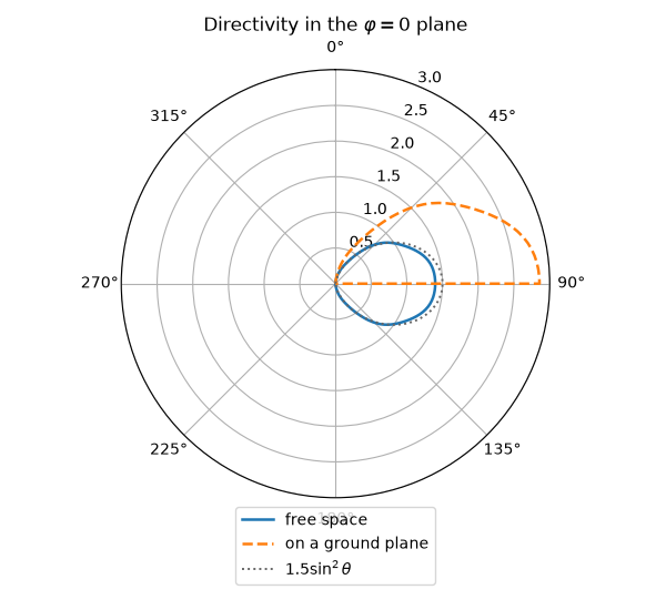
Closing the bottom face with PEC and standing the filament on it turns the dipole into a monopole. Nothing about the source changes: the same current, on a path that now starts at the wall. Image theory does the rest — the far-field monitor leaves the box open on that face and completes it with the mirror image, so the pattern is masked below the plane and the horizon directivity doubles.

grounded = dict(OPEN, zmin="PEC")
model = air_box(grounded, z0=0.0, height=HALF)
model.add_source(sources.SourceCurrentPath(name="mono", path=[(0, 0, 0.0), (0, 0, LENGTH)]))
monopole = radiate(model, "mono")

p_mono = ETA0 * (k * LENGTH) ** 2 / (3.0 * np.pi)
print(f"ground plane: P_rad / monopole  {monopole.P_rad / p_mono:.3f}   (target 1.00 +- 0.05)")
print(f"ground plane: peak directivity  {monopole.directivity.max():.3f}   (3.00, see below)")

  mesh | feature planes
  mesh | grid lines
  mesh | materials
  mesh | conformal cells
  mesh | PEC masks
  mesh | 92 x 92 x 49 cells
ground plane: P_rad / monopole  0.960   (target 1.00 +- 0.05)
ground plane: peak directivity  3.135   (3.00, see below)

Both powers hold to a few percent, which is the number that matters: the current that reached the grid is the current that was asked for. The monopole radiates half the power of the two-sided dipole it images into, into half the solid angle — hence twice the free-space power for the same current, and twice the directivity.

The directivities come out three to four percent high. That excess is not the source but the near-to-far-field transform, which reads a cubic box and converges towards the exact pattern only as the box is sampled more finely; power_balance near 1 says the transform is at least self-consistent. Read the overlay below as the shape check it is, and the radiated power as the calibration.

fig, ax = plt.subplots(figsize=(6.0, 5.5), subplot_kw={"projection": "polar"})
for pattern, label, style in (
    (dipole, "free space", "-"),
    (monopole, "on a ground plane", "--"),
):
    cut = pattern.directivity[:, 0]
    ax.plot(pattern.theta, cut, style, lw=1.8, label=label)
ax.plot(
    dipole.theta,
    1.5 * np.sin(dipole.theta) ** 2,
    ":",
    color="0.4",
    lw=1.4,
    label=r"$1.5\sin^2\theta$",
)
ax.set_theta_zero_location("N")
ax.set_theta_direction(-1)
ax.set_title("Directivity in the $\\varphi = 0$ plane")
ax.legend(loc="lower center", bbox_to_anchor=(0.5, -0.22))
fig.tight_layout()

Paths that are not straight

path takes any Curve, so a coil is a helix and a loop a pair of arcs chained into a closed curve. A closed path is a magnetic dipole: no charge accumulates anywhere, and the pattern is the dipole’s turned on its side.

from magnelio import geo

a = 4e-3
loop = geo.Curve.arc((a, 0, 0), (-a, 0, 0), (0, -a, 0)).joined(
    geo.Curve.arc((0, -a, 0), (a, 0, 0), (0, a, 0))
)
model.add_source(sources.SourceCurrentPath(name="loop", path=loop))

A curved path is walked as a staircase across the cells, which costs nothing in the dipole moment — the staircase runs monotonically from end to end, so its signed steps sum to the exact chord — but does ask for enough cells across the curve if the finer structure of the field matters.

What to watch

• The current is prescribed, not solved for. Nothing the model does changes I(t). That is the right description of a driven coil or a known interference current, and the wrong one for an antenna whose current distribution is the answer you are after — feed that with a port.

• The amplitude is in amperes, and reads as an effective value in the frequency domain, like every other amplitude in the library. source.amplitude_unit says so.

• Edges held at zero take no current. A path inside a perfect conductor, or running along a PEC wall, radiates less than asked; the source warns instead of doing it quietly. Currents on a conductor belong on a port or a lumped element.

• Give the far-field box room. A dipole’s reactive near zone reaches about \(\lambda / 2\pi\); with less than half a wavelength of clearance the near-to-far-field transform stops closing, and power_balance says by how much.

• Under a symmetry declaration the mesh is the kept half. Give the path in that half and let the symmetry wall supply its image.

plt.show()