Watching a simulation that is still running

A run that takes an hour raises one question every few minutes: what is it doing? The progress line in the terminal that started it answers for that terminal; a colleague’s notebook, a laptop at home, or the same notebook after the kernel was restarted all need another way in.

The recipe has two halves. The analysis is given a project= directory, and streams into it as it marches — every energy sample, every port signal, the run’s state. Any other process then opens that directory and lets the project report: as a table that moves, as a picture of the stored energy, or as a live panel in a notebook.

import os
import tempfile
import threading
import time

import magnelio as mio
from magnelio import geo, ports

A run to watch

The structure does not matter for this page. A length of WR-90 waveguide with a port at each end is enough to make the solver march for a few seconds, which is all the following needs.

a, b, length = 22.86e-3, 10.16e-3, 60e-3
model = mio.GeometryModel(background="pec", boundary_conditions=mio.BoundaryConditions())
model.add(geo.Brick(origin=(-a / 2, -b / 2, 0), size=(a, b, length), material="air"))
model.add_port(ports.PortWaveguide(name="p1", plane="zmin"))
model.add_port(ports.PortWaveguide(name="p2", plane="zmax"))
mesh = mio.Mesh.from_geometry(
    model, mio.MeshControl(max_cell_size=b / 12), f_max=12e9, verbose=False
)

proj_dir = os.path.join(tempfile.mkdtemp(), "wr90")

The solver, somewhere else

On a real job the solver runs in another process — a batch job on a cluster, a second notebook, a script left running overnight. This page has to stay inside one interpreter, so the solver runs on a thread here; the reader below opens the directory and sees nothing but the files, exactly as a second process would.

def solve():
    analysis = mio.AnalysisScatteringTD(mesh=mesh, f_min=8e9, project=proj_dir, verbose=False)
    analysis.run(excited=["p1"])


job = threading.Thread(target=solve)
job.start()
while not os.path.exists(os.path.join(proj_dir, "project.json")):
    time.sleep(0.05)

Following the run

open_project() opens the directory; watch() looks at it every interval seconds and hands the project back whenever something changed — a run starting, a new energy sample, a run ending — until the project is finished. Each report here is one line: the status, the step the solver has reached, and the stored energy in dB below its peak, which is the number the run’s stop criterion watches.

proj = mio.open_project(proj_dir)
for snapshot in proj.watch(interval=0.25):
    run = snapshot.runs.get("p1_mode0")
    if run is None or run.state == "pending":
        print(f"{snapshot.status:8s}  planned")
        continue
    level = "—" if run.energy_db is None else f"{run.energy_db:6.1f} dB below peak"
    print(f"{snapshot.status:8s}  step {run.n_steps:6d}  {level}")

job.join()

running   planned
running   step    601     0.0 dB below peak
running   step   1501   -47.7 dB below peak
running   step   2401   -57.8 dB below peak
running   step   3301   -63.2 dB below peak
running   step   4201   -67.0 dB below peak
done      step   5101   -70.1 dB below peak

The loop body prints what it wants seen — inside a loop a bare expression such as run.energy_db shows nothing, in a notebook as anywhere else. When the whole table is what you want, follow() is that loop ready-made: it shows the summary at every change and replaces it in place instead of scrolling — in a notebook the cell output is cleared and redrawn, on a terminal the table is redrawn over its own lines. On a finished project it shows the final state once: what ran, how long it took, and why each run stopped.

follow(plot=True) adds the energy plot below the table, redrawn with it — a figure drawn inside a loop of your own would not show until the cell ends, because the notebook’s inline backend flushes a cell’s figures when the cell is over. plot= also takes a callable draw(project, ax) for a picture of your own, with your own axis limits.

proj.follow(interval=0.25)

Project /tmp/tmpd0j04vta/wr90
  analysis   AnalysisScatteringTD
  status     done
  last call  started 2026-09-09 09:38:56, 2.8 s ago
  created    2026-09-09 09:38:56
  runs       1
run       excited  state  steps    energy  elapsed  stop reason
────────  ───────  ─────  ─────  ────────  ───────  ───────────
p1_mode0  p1:0     done    5101  -70.1 dB    1.4 s  energy

Project /tmp/tmpd0j04vta/wr90

analysis	AnalysisScatteringTD
status	done
last call	started 2026-09-09 09:38:56, 2.8 s ago
created	2026-09-09 09:38:56
runs	1

run	excited	state	steps	energy	elapsed	stop reason
p1_mode0	p1:0	done	5101	-70.1 dB	1.4 s	energy

The picture behind the line

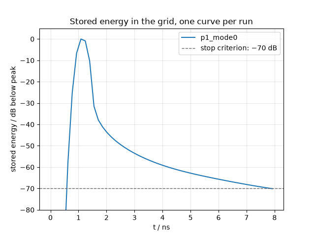
plot_energy draws every run’s stored energy in dB below its peak — the same figure the progress line and the table report, over the whole run — with the energy criterion as a dashed line. On a project that is still marching it shows the curve so far; repeat the cell to see it grow.

fig, ax = proj.plot_energy()
ax.set_title("Stored energy in the grid, one curve per run")

Text(0.5, 1.0, 'Stored energy in the grid, one curve per run')

A panel that keeps itself current

In a notebook, proj.monitor() returns a widget: the run table above the energy plot, refreshed from a background thread every few seconds until the project is finished. Leave it as the last expression of a cell; the cell returns at once and the panel keeps moving while you work in other cells. It needs the jupyter extra (pip install 'magnelio[jupyter]'), and it is a notebook thing — this page is built without one, so the panel is only assembled here, not shown.

try:
    panel = proj.monitor(interval=2.0)
except ImportError:
    panel = None
else:
    panel.stop()

Doing something at every change

Anything that should happen whenever the store changes — redraw a figure, append a line to a log, push a message — is a callable handed to watch(on_change=...). The loop then runs inside watch, which returns the project when the run is finished:

changes = []
mio.open_project(proj_dir).watch(interval=0.25, on_change=lambda p: changes.append(p.status))
print(f"{len(changes)} report(s) on a finished project; the last says {changes[-1]!r}")

1 report(s) on a finished project; the last says 'done'

What to remember

• ``project=`` is the switch. Without it a run lives in the memory of the process that computes it; with it, everything lands on disk as it happens, and any process may look.

• The project reads itself. A project that is not finished re-reads its index whenever the file changes, so typing proj again shows the current state — no refresh() needed while it marches.

• ``watch`` polls, on purpose. Every energy sample goes to disk at once and the index is replaced atomically, so a poll every few seconds sees everything and works on any file system a batch job might write to; there is nothing to subscribe to.

• One number to look at. Stored energy in dB below the peak is what the stop criterion watches, what the progress line shows, what the table lists and what plot_energy draws.

• A dead run reads ``stale``. A run whose solver process no longer exists on this host is not running; watch ends on it the way it ends on done.