Lumped port tuning: microstrip

A pre-flight check for a lumped port terminating a microstrip: fill in the given quantities of your target model, run, and the scoreboard tells you how good the termination is — worst reflection, usable band, phase error. Edit the knobs and re-run until the numbers meet your spec, then carry the settings over.

The microstrip termination is a vertical lumped port from the end of the trace straight down to the ground plane, so there is no gap-length knob — the knobs are the trace-end position and the port impedance. Because the line is dispersive, the position compromise is frequency-dependent: pick it for the part of the band that matters most. The page Lumped ports: investigations explains the measurement and shows the sweeps; every number here is a property of your grid.

import matplotlib.pyplot as plt
import numpy as np

import magnelio as mio
from magnelio import geo, plots, ports

Given quantities

The cross-section of the target model — substrate, trace, shield — plus band and resolution. Copy the resolution your production mesh will actually have around the trace.

h_sub = 0.8e-3  # substrate height [m]
w_strip = 1.2e-3  # trace width [m]
t_met = 0.2e-3  # metallisation thickness [m]
eps_r = 4.3  # substrate permittivity (FR4)
W_box = 8.0e-3  # shield width [m]
H_box = 5.0e-3  # shield height [m]
f_max = 15e9  # upper band edge [Hz]
n_per_lambda = 25  # mesh resolution [cells per wavelength]

The knobs

• end_position — where the trace ends relative to the reference plane (negative = before it); sets the phase error.

• z0_port — None uses the line impedance of the grid from the waveguide-port solver; a number uses that instead.

end_position = 0.0
z0_port = None

Derived quantities

L = 5.0 * w_strip  # waveguide port to reference plane [m]
tail = 2.5 * h_sub  # substrate/air continuing beyond the trace end [m]

Measurement machinery — the shielded microstrip, once as a plain through line (the phase reference) and once ending in the candidate termination, with substrate and air continuing for a short tail behind the trace end as they would in a real layout.

def _model(length, strip_len):
    fr4 = mio.Material.from_isotropic(name="FR4", epsilon=eps_r)
    model = mio.GeometryModel(background="pec")
    model.add(geo.Brick(origin=(-W_box / 2, 0.0, 0.0), size=(W_box, h_sub, length), material=fr4))
    air = geo.Brick(
        origin=(-W_box / 2, h_sub, 0.0), size=(W_box, H_box - h_sub, length), material="air"
    )
    strip = geo.Brick(
        origin=(-w_strip / 2, h_sub, 0.0), size=(w_strip, t_met, strip_len), material="pec"
    )
    model.add(geo.Difference(air, strip))
    model.add(strip)
    model.add_port(ports.PortWaveguide(name="wg", plane="zmin", n_modes=1))
    return model


def _mesh(model):
    return mio.Mesh.from_geometry(
        model,
        mio.MeshControl(min_nodes_per_wavelength=n_per_lambda),
        f_max=f_max,
    )


ref_model = _model(L, strip_len=L)
ref_model.add_port(ports.PortWaveguide(name="far", plane="zmax", n_modes=1))
ref = mio.AnalysisScatteringTD(mesh=_mesh(ref_model), verbose=False).run(excited=[("wg", 0)])

z_pin = L + end_position
model = _model(z_pin + tail, strip_len=z_pin)
mesh = _mesh(model)
z_line = mio.AnalysisScatteringTD(mesh=mesh, verbose=False).solve_ports()["wg"].modes[0].z_line
print(f"line impedance on this grid: {z_line:.2f} Ohm")

model.add_port(
    ports.PortLumped(
        name="dut",
        start=(0.0, h_sub, z_pin),
        end=(0.0, 0.0, z_pin),
        Z0=float(z0_port if z0_port is not None else z_line),
    )
)
result = mio.AnalysisScatteringTD(mesh=mesh, ports=list(model.ports), verbose=False).run(
    excited=[("wg", 0)]
)

  mesh | feature planes
  mesh | grid lines
  mesh | materials
  mesh | conformal cells
  mesh | PEC masks
  mesh | 24 x 23 x 16 cells
  mesh | feature planes
  mesh | grid lines
  mesh | materials
  mesh | conformal cells
  mesh | PEC masks
  mesh | 24 x 23 x 22 cells
line impedance on this grid: 50.23 Ohm

The test fixture

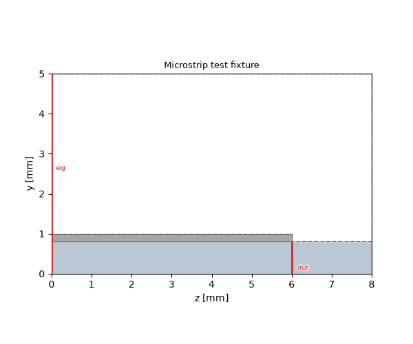
A cut along the propagation direction, through the trace centre: the waveguide port on the left, the trace ending at end_position relative to the reference plane, the vertical lumped port from the trace end down to the ground plane, and the substrate/air tail continuing to the shield’s back wall.

fig, ax = plots.plot_cross_section(model, "x", 0.0, flip=True, title="Microstrip test fixture")

The scoreboard

The phase error is polarity-normalised: the sign of a mode profile is a convention, so the error is referenced to the nearest multiple of 180° at the low end of the band.

f = np.asarray(result.f_axis)
band = f <= f_max
s11_db = result.db("wg", "wg")
err = result.phase("dut", "wg") - ref.phase("far", "wg")
err -= 180.0 * np.round(err[int(np.argmax(f >= f_max / 15.0))] / 180.0)

good = s11_db[band] < -20.0
f_edge = f[band][np.argmin(good)] if not good.all() else f[band][-1]
print("--- current settings — tune until this meets your spec ---")
print(f"worst |S11| in band : {s11_db[band].max():6.1f} dB")
print(f"|S11| < -20 dB up to: {f_edge / 1e9:6.2f} GHz")
print(f"max |phase error|   : {np.abs(err[band]).max():6.2f} deg")

fig, (ax1, ax2) = plt.subplots(1, 2, figsize=(9.0, 3.6))
ax1.plot(f[band] / 1e9, s11_db[band])
ax1.set_xlabel("frequency [GHz]")
ax1.set_ylabel("|S11| [dB]")
ax1.set_title("Self-reflection")
ax1.grid(True, alpha=0.3)
ax2.plot(f[band] / 1e9, err[band])
ax2.set_xlabel("frequency [GHz]")
ax2.set_ylabel("phase error [deg]")
ax2.set_title("Phase error at the reference plane")
ax2.grid(True, alpha=0.3)
fig.tight_layout()

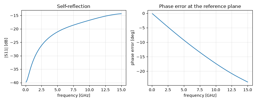
--- current settings — tune until this meets your spec ---
worst |S11| in band :  -14.4 dB
|S11| < -20 dB up to:   5.97 GHz
max |phase error|   :  23.73 deg

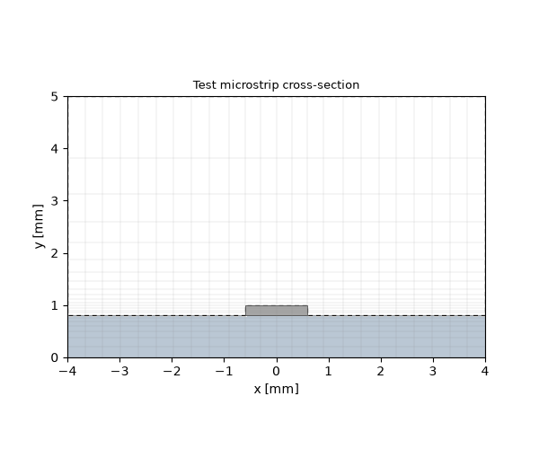
The cross-section with the mesh it is actually solved on.

fig, ax = plots.plot_cross_section(
    model, "z", L / 2, mesh=mesh, title="Test microstrip cross-section"
)

Carry it over

Transfer end_position (relative to where your reference plane is) and the port impedance into the target model once the numbers meet your spec. Background and sweeps: Lumped ports: investigations. When the cross-section, resolution or band changes, run this page again.