Note
Go to the end to download the full example code.
Your first simulation: a parallel-plate line#
This tutorial walks through one complete Magnelio workflow — geometry, materials, boundary conditions, mesh, waveguide ports, time-domain run, broadband S-parameters — on the simplest structure that has all of these ingredients: a short section of parallel-plate transmission line.
The structure is deliberately trivial so that every number the solver produces can be checked against a closed-form result. At the end we compare the computed line impedance and the transmission phase against the textbook values.
The problem#
Two perfectly conducting plates of width a, separated by an air
gap b, guide a TEM wave: the electric field points from plate to
plate, the magnetic field lies parallel to the plates, and the wave
propagates along the line at the speed of light — at every frequency,
because a TEM mode has no cut-off. For plates that are wide compared
to the gap, the line impedance approaches the textbook value
with \(\eta_0 \approx 376.73\,\Omega\) the impedance of free space. We model the ideal limit exactly by closing the two open sides with magnetic walls (PMC): they force the field to stay purely vertical, as if the plates were infinitely wide. This trick — a symmetry wall standing in for a continuation of the structure — is a workhorse of practical EM modelling, and this is the smallest example of it.
We simulate a line with a = 10 mm, b = 5 mm, length
L = 20 mm, up to 10 GHz. The first higher-order mode of this
cross-section appears near 15 GHz, so over the whole simulated band
exactly one mode propagates and the S-parameters are the plain
two-port quantities S11 and S21.
Imports: the core and the domains#
Every Magnelio script starts with the same three lines. The core
magnelio namespace — model container, mesh, boundary
conditions, the analyses — is imported once under the short alias
mio. The domain namespaces (geo for solids and
booleans, ports, plots, …) come
in as their own names and are picked up at the call site — no need
to decide up front which primitives the model will use. The
physical constants are four curated symbols (C0, EPS0,
MU0, ETA0), so a star import is safe and keeps formulas
readable.
import matplotlib.pyplot as plt
import numpy as np

import magnelio as mio
from magnelio import geo, plots, ports
from magnelio.constants import *

a = 10e-3  # plate width [m]
b = 5e-3  # plate spacing [m]
L = 20e-3  # line length [m]
f_max = 10e9  # upper band edge [Hz]
Geometry, materials and boundary conditions#
A Magnelio model is a GeometryModel filled with
shapes, each carrying its Material — built-in
materials are simply named by string ("air", "pec",
"vacuum"); only parameterised materials need an explicit
Material object. Our entire
geometry is a single air-filled Brick;
the conductors do not need to be drawn at all, because they coincide
with the boundary of the computational domain:
the
yfaces are the plates themselves → PEC (the default),the
xfaces are the idealising magnetic walls → PMC,the
zfaces will carry the two ports.
The boundary closure is declared once, on the model, and travels with the mesh from there.
model = mio.GeometryModel(
    boundary_conditions=mio.BoundaryConditions(xmin="PMC", xmax="PMC"),
)
model.add(
    geo.Brick(origin=(-a / 2, -b / 2, -L / 2), size=(a, b, L), material="air"),
)
GeometryModel(1 shapes, background=air)
Ports#
A PortWaveguide is the declarative “this
face is a waveguide cross-section” statement: at each z end of
the line the solver will find the guided modes of the cross-section,
use them to launch the excitation, and absorb whatever comes back.
With n_modes=1 each port handles the fundamental (here: TEM)
mode.
model.add_port(ports.PortWaveguide(name="port1", plane="zmin", n_modes=1))
model.add_port(ports.PortWaveguide(name="port2", plane="zmax", n_modes=1))
GeometryModel(1 shapes, background=air)
Mesh#
Mesh.from_geometry builds a
hexahedral grid resolving the geometry and the shortest wavelength of
the requested band. A featureless air box would be meshed very
coarsely — perfectly stable, but port quantities converge with
resolution like every discrete result. The
MeshControl knobs override such decisions; here we
cap the cell size at 1/16 of the plate spacing.
mesh = mio.Mesh.from_geometry(
    model,
    mio.MeshControl(max_cell_size=b / 16),
    f_max=f_max,
)
print(f"grid: {mesh.Nx} x {mesh.Ny} x {mesh.Nz} cells")
  mesh | feature planes
  mesh | grid lines
  mesh | materials
  mesh | materials | done (19.8 s)
  mesh | conformal cells
  mesh | conformal cells | done (7.7 s)
  mesh | PEC masks
  mesh | 32 x 16 x 64 cells (27.7 s total)
grid: 32 x 16 x 64 cells
Looking at geometry and mesh before spending any solver time is one
call each. model.show() is the 3D view: the model opened along a
cutting plane, with the grid cells the cut exposes coloured by the
material the mesher assigned. In the notebook version of this
tutorial it is an interactive widget (orbit, pan, zoom, and the
cutting plane in its toolbar); here it is rendered as a picture.
model.show(mesh=mesh, cut=("y", 0.0))
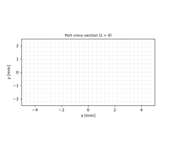
The 2D cross-section is the exact companion — a section through the CAD model with the grid lines overlaid.
The port modes#
The analysis object bundles mesh, band and ports — f_max is
taken from the mesh, which records the design frequency it was
generated for. Solving the port
modes is a cheap 2D eigenproblem — worth inspecting before the 3D
run. The report prints the mode ladder of each port; for a TEM mode
it also carries the line impedance, which we can hold against the
textbook formula.
analysis = mio.AnalysisScatteringTD(mesh=mesh, verbose=False)

report = analysis.solve_ports()["port1"]
print(report)

z_line = report.modes[0].z_line
z_analytic = ETA0 * b / a
print(f"Z_L (port solver): {z_line:9.4f} Ohm")
print(f"Z_L (eta0 * b/a) : {z_analytic:9.4f} Ohm")
print(f"relative deviation: {abs(z_line / z_analytic - 1):.2e}")
Port 'port1' — 1 mode(s)
  z_line = 188.37 Ω (on this grid)
  [0] TEM_lap00    TEM f_c = 0.0000 GHz  z_line = 188.37 Ω  ε_eff = 1.000  termination = dtbc (chain floor <= -329 dB)
Z_L (port solver):  188.3652 Ohm
Z_L (eta0 * b/a) :  188.3652 Ohm
relative deviation: 1.11e-16
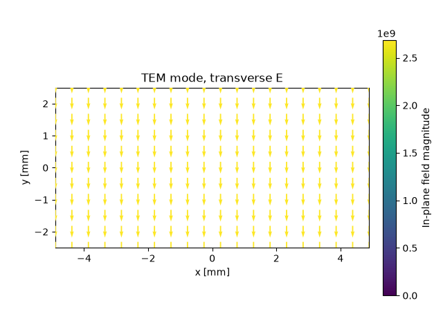
The two agree to machine precision: the uniform TEM field of this cross-section is represented exactly on the grid. (On less trivial cross-sections the discrete impedance converges with mesh resolution instead — one of the reasons to look at port reports before trusting a result.)
The transverse mode profile confirms what a TEM plate mode should look like — a uniform vertical E field:
Run and S-parameters#
run performs the time-domain simulation: port 1 launches a
broadband pulse, the fields propagate through the line, both ports
record what arrives, and the recorded signals are transformed into
S-parameters over the whole band — one run, all frequencies. The
run stops on its own once the port signals have decayed.
result = analysis.run(excited=[("port1", 0)])

f = result.f_axis
s11_db = result.db("port1", "port1")
s21_db = result.db("port2", "port1")

fig, ax = plt.subplots()
ax.plot(f / 1e9, s11_db, label="|S11|")
ax.plot(f / 1e9, s21_db, label="|S21|")
ax.set_xlabel("frequency [GHz]")
ax.set_ylabel("magnitude [dB]")
ax.set_title("Parallel-plate line, 20 mm")
ax.grid(True)
ax.legend()

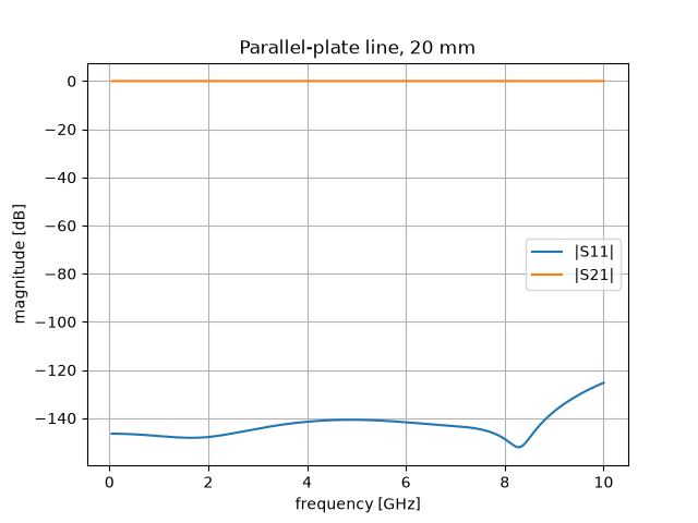
print(f"max |S11| in band: {s11_db.max():6.1f} dB")
max |S11| in band: -125.3 dB
A matched, lossless, uniform line transmits everything: |S21|
sits at 0 dB and |S11| at the numerical noise floor (below
-120 dB) — the
ports launch and absorb the TEM wave without spurious reflection.
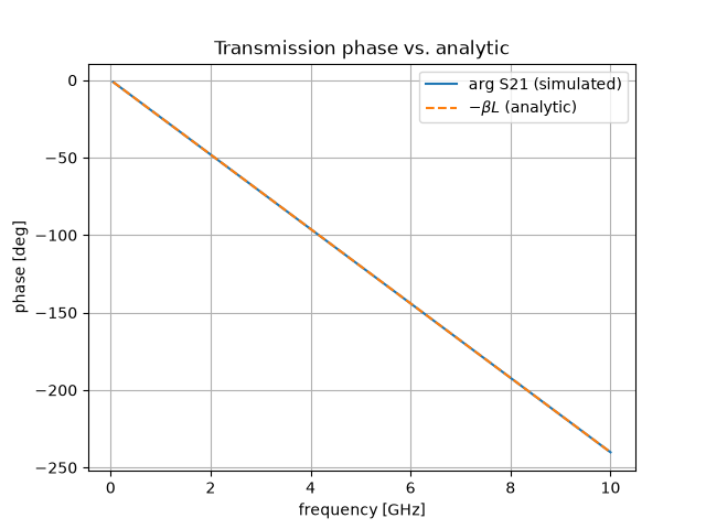
The phase of S21 carries the physics of the 20 mm flight path. For a TEM line it must follow \(e^{-j \beta L}\) with \(\beta = 2 \pi f / c_0\):
s21 = result.S("port2", "port1")
phase_sim = np.unwrap(np.angle(s21))
phase_ref = -2 * np.pi * f / C0 * L

fig, ax = plt.subplots()
ax.plot(f / 1e9, np.degrees(phase_sim), label="arg S21 (simulated)")
ax.plot(f / 1e9, np.degrees(phase_ref), "--", label=r"$-\beta L$ (analytic)")
ax.set_xlabel("frequency [GHz]")
ax.set_ylabel("phase [deg]")
ax.set_title("Transmission phase vs. analytic")
ax.grid(True)
ax.legend()

print(f"max phase deviation: {np.degrees(np.abs(phase_sim - phase_ref)).max():.3f} deg")
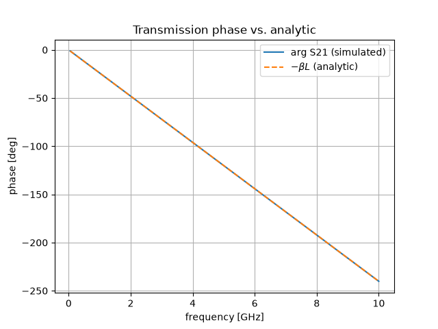
max phase deviation: 0.033 deg
Where to go next#
You have seen the complete standard workflow: geometry → boundary conditions → ports → mesh → run → S-parameters, plus the two habits worth keeping — inspect cross-sections and port reports before the run, and validate against known results where they exist. The next tutorial builds a real three-dimensional structure (a coaxial line) from solids and boolean operations, with a port spec matched to its cross-section.
Total running time of the script: (0 minutes 44.396 seconds)