Using disk storage: monitors at scale, resume, ParaView

Everything so far lived in RAM: results and monitor data existed as long as the Python session and vanished with it — and a monitor held only the run it had just witnessed. This tutorial gives a simulation a project directory instead. The model, every run’s port signals, every monitor’s data and a resumable checkpoint all stream to disk while the solver marches; evaluation becomes a separate step that can happen in another script, on another day — or in ParaView.

The device is the magic tee from the previous tutorial, this time carrying a full-volume 3D field monitor — exactly the kind of data you do not want to keep in memory, and the kind ParaView is made for.

The tee again, in one block

Geometry, ports and mesh are unchanged from the previous tutorial — three WR-90 arms united into a tee, four single-mode ports, and the band-limited 8.2–12.4 GHz excitation.

import os
import tempfile

import matplotlib.pyplot as plt
import numpy as np

import magnelio as mio
from magnelio import geo, monitors, ports

a = 22.86e-3  # WR-90 broad wall
b = 10.16e-3  # WR-90 narrow wall
arm = 30.0e-3  # arm length beyond the junction

collinear = geo.Brick(
    origin=(-(a / 2 + arm), -a / 2, 0.0), size=(a + 2 * arm, a, b), material="air"
)
h_arm = geo.Brick(origin=(-a / 2, 0.0, 0.0), size=(a, a / 2 + arm, b), material="air")
e_arm = geo.Brick(origin=(-b / 2, -a / 2, 0.0), size=(b, a, b + arm), material="air")

model = mio.GeometryModel(background="pec")
model.add(geo.Union(collinear, h_arm, e_arm, name="tee"))
model.add_port(ports.PortWaveguide(name="port1", plane="xmin", n_modes=1))
model.add_port(ports.PortWaveguide(name="port2", plane="xmax", n_modes=1))
model.add_port(ports.PortWaveguide(name="port3", plane="ymax", n_modes=1))
model.add_port(ports.PortWaveguide(name="port4", plane="zmax", n_modes=1))

f_min, f_max = 8.2e9, 12.4e9

mesh = mio.Mesh.from_geometry(
    model,
    mio.MeshControl(min_nodes_per_wavelength=15, min_cell_size=1.59e-3),
    f_max=f_max,
)

mesh | feature planes
mesh | grid lines
mesh | materials
mesh | conformal cells
mesh | PEC masks
mesh | 48 x 32 x 24 cells

A 3D monitor and a project directory

The monitor spans the whole domain this time — omitting corners records everywhere — and accumulates the complex E and H fields at 10 GHz. On an in-RAM run a volume monitor is the fastest way to fill your memory; on a project run its data streams to disk.

Memory is not the only thing it spends. Left alone, the running DFT takes a contribution from every cell at every time step, which on this model costs as much again as the solve itself. interval thins that sampling, and the accuracy it trades away is bounded by how many samples per period of the highest frequency in the band remain: at twelve, this run lands on every second step and the recorded field moves by 2e-5. Sizing the interval from f_max rather than from the monitor’s own 10 GHz is the safe habit — anything the fields carry above the resulting Nyquist frequency would fold onto the recorded bin.

The project itself is just a directory path. Here it goes to a temporary folder so this page can build anywhere; in real work you would pick a permanent location on fast local storage, because the solver writes into it continuously.

volume = monitors.MonitorFieldFrequency(
    freqs=[10.0e9],
    fields=["E", "H"],
    interval=1.0 / (12 * f_max),
    name="volume_pattern",
)

proj_dir = os.path.join(tempfile.mkdtemp(), "magic_tee")

analysis = mio.AnalysisScatteringTD(
    mesh=mesh,
    f_min=f_min,
    monitors=(volume,),
    project=proj_dir,
    geometry=model,
    verbose=False,
)

result = analysis.run(excited=["port3", "port4"], port_signal_stop_db=50.0)
print(type(result).__name__, "->", result.status)

Project -> done

run() on a project returns not an in-RAM result but a reader over the directory it just wrote. Both excitations now live on disk as separate named runs — including, unlike in the previous tutorial, both sets of monitor data. A look at the files shows where everything went (sizes in kB):

for root, _dirs, files in sorted(os.walk(proj_dir)):
    rel = os.path.relpath(root, proj_dir)
    prefix = "" if rel == "." else rel + "/"
    for name in sorted(files):
        size = os.path.getsize(os.path.join(root, name))
        print(f"{prefix + name:<58} {size / 1e3:9.1f}")

geometry.brep                                                    9.9
geometry.json                                                    0.8
mesh.h5                                                      11787.6
project.json                                                     3.8
runs/port3_mode0/checkpoint.h5                                1523.7
runs/port3_mode0/fields_freq.h5                               5579.0
runs/port3_mode0/results.h5                                    699.6
runs/port4_mode0/checkpoint.h5                                1523.7
runs/port4_mode0/fields_freq.h5                               5579.0
runs/port4_mode0/results.h5                                    699.6

project.json carries the run registry and the reconstruction recipe, mesh.h5 and geometry.brep the exact model, and each run directory holds its streamed port signals (results.h5), the monitor’s frequency-domain volume (fields_freq.h5) and a resumable checkpoint.h5.

Evaluating from disk — in a different session

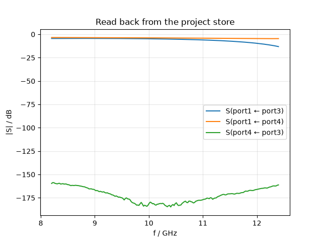
The reader that run() returned is the same object any other process gets from magnelio.open_project() — nothing below needs the analysis, the mesh, or the solver. This is the separation the store exists for: a cluster job computes, your laptop evaluates. S-parameters are derived on read from the stored signals, with the accessors you already know:

# ``open_project`` hands back the very same kind of object ``run()``
# returned above — a reader over the directory — only initialised from
# the path instead of by the run that wrote it.
result_loaded = mio.open_project(proj_dir)
print(type(result_loaded).__name__, "->", result_loaded.status)

fig, ax = result_loaded.plot_s(("port1", "port3"), ("port1", "port4"), ("port4", "port3"))
ax.set_title("Read back from the project store")

Project -> done

Text(0.5, 1.0, 'Read back from the project store')

Watching a run: the energy trace

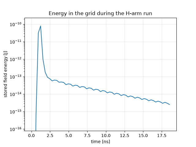
Alongside the port signals the store keeps the total field energy in the grid, sampled whenever the solver checks its stopping criterion. plot_energy draws it for every run, in dB below the run’s peak — the number the progress line reports and the stop criterion watches — with that criterion as a dashed line. The curve is the clearest single picture of what a time-domain run does: the excitation pumps energy in, the ports carry it out, and the run ends when what remains has fallen far enough below the peak.

This is also the trace to watch while a long simulation is still running. Each sample is flushed to disk as it is taken, so a second process — another shell, a notebook on your laptop — can open_project() the very same directory and follow the run live, without touching the job that is computing; the how-to Watching a simulation that is still running shows the loop, and the live panel for a notebook.

fig, ax = result_loaded.plot_energy()
ax.set_title("Energy in the grid during the two runs")

trace = result_loaded.runs["port3_mode0"].energy_trace
print(f"energy samples stored for the H-arm run: {len(trace)}")

energy samples stored for the H-arm run: 65

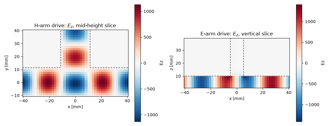
The monitor data of every run is preserved — where the previous tutorial had to harvest its in-RAM monitors between two run() calls, the store keeps both volumes side by side, and monitors_for picks a run by its excitation. Because the stored pattern is a full 3D volume, the slice plane is chosen at plot time, not at declaration time — the H-arm drive on the mid-height cut, the E-arm drive on the vertical cut, both from data recorded in the same simulation:

mon_h = result_loaded.monitors_for(("port3", 0))["volume_pattern"]
mon_e = result_loaded.monitors_for(("port4", 0))["volume_pattern"]

fig, axes = plt.subplots(1, 2, figsize=(11, 4.2))
mon_h.plot(
    component="Ez", normal="z", position=b / 2, plot_type="color", geometry=model, ax=axes[0]
)
mon_e.plot(component="Ez", normal="y", position=0.0, plot_type="color", geometry=model, ax=axes[1])
axes[0].set_title("H-arm drive: $E_z$, mid-height slice")
axes[1].set_title("E-arm drive: $E_z$, vertical slice")
fig.tight_layout()

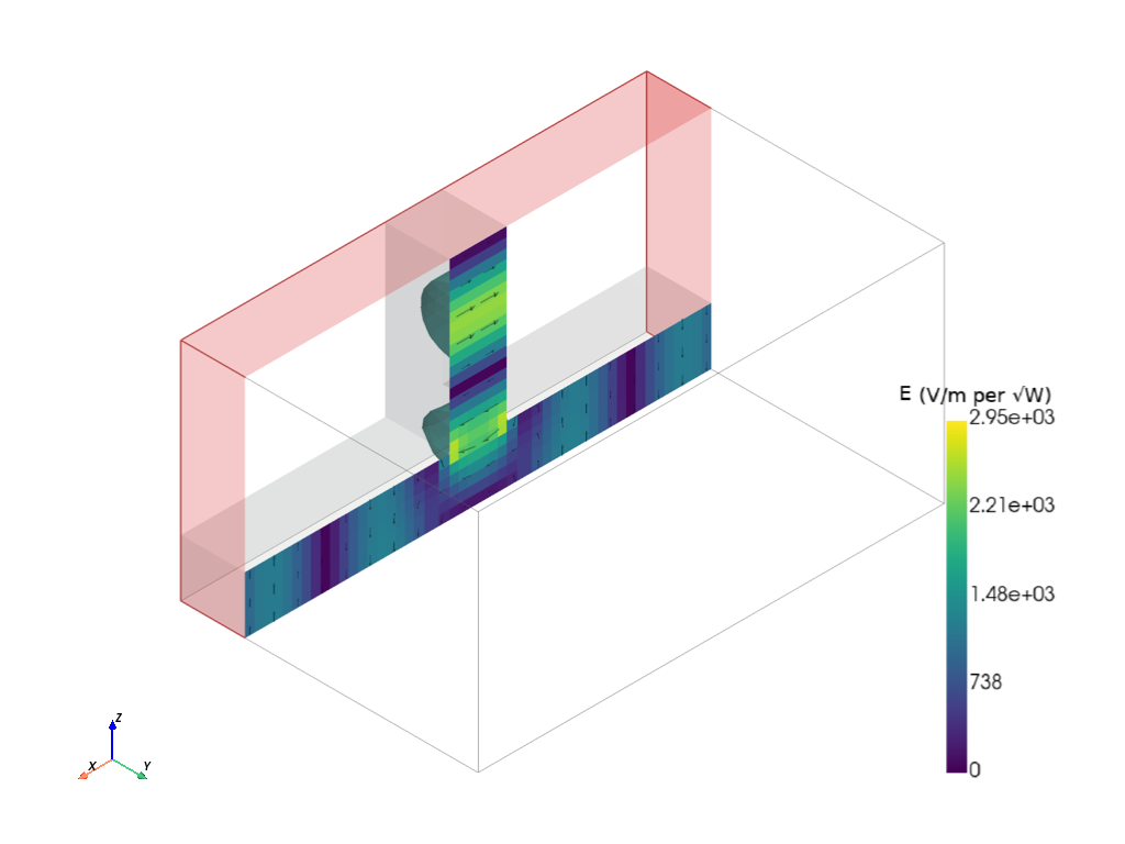
The volume can also be opened in the 3D viewer. show lays the field on the viewer’s cutting plane — here the E-arm drive, cut along the E-arm’s own symmetry plane, the tee’s metal drawn with it and the cells inside the walls cut out of the field sheet — and, with volume="isosurface", adds the surface where the magnitude of E reaches half its ceiling, clipped at the cut so its inside shows. In a notebook the position slider walks the cut through the whole recorded volume, a phase slider turns the complex pattern, a level slider moves the surface, and the Show menu swaps the arrows on the cut for arrows on a lattice through the volume; a documentation build shows the frame the call asks for.

mon_e.show(
    component="E",
    normal="y",
    position=0.0,
    geometry=model,
    mesh=mesh,
    phase=90.0,
    volume="isosurface",
)

Static Scene

Interactive Scene

Running longer: resume

Every run directory carries a checkpoint with the complete solver state, written periodically and at the end of the run. magnelio.resume() rebuilds the run from the stored recipe, loads that checkpoint and continues the same trajectory — no seam, no restart. That is the answer to three situations: a crashed or interrupted job, a stop criterion chosen too shallow, and the convergence question “would more ring-down change my S-parameters?”. Here we ask the third one, extending the H-arm run by 2000 steps:

s13_before = result_loaded.S("port1", "port3")
n_before = result_loaded.runs["port3_mode0"].n_steps

result_resumed = mio.resume(
    proj_dir, excited="port3", total_time_steps=n_before + 2000, verbose=False
)

s13_after = result_resumed.S("port1", "port3")
print(f"steps: {n_before} -> {n_before + 2000}")
print(f"max |dS13| from 2000 extra steps: {np.abs(s13_after - s13_before).max():.1e}")

steps: 6401 -> 8401
max |dS13| from 2000 extra steps: 3.7e-04

The change is far below any engineering tolerance — the original stop criterion was deep enough, and finding that out cost two thousand time steps instead of a rerun. (A resumed run appends to the same streams, the monitor volume along with them.)

Into ParaView

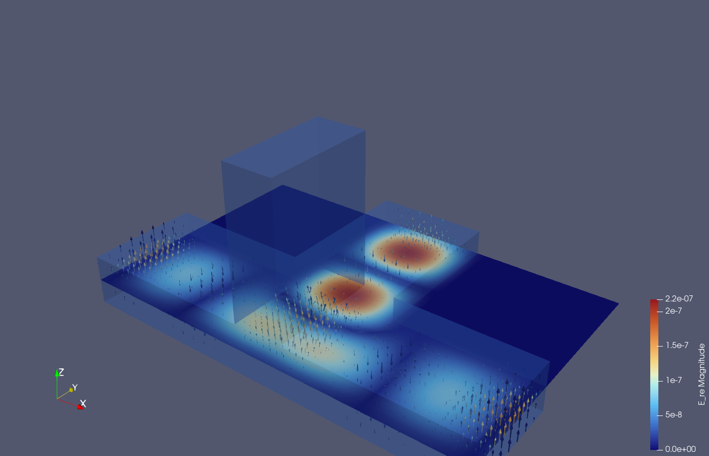
Slice plots answer questions you already know how to ask; a 3D volume invites the ones you don’t. A project run can be handed to ParaView as a ready-made session — an export you ask for, since the VTK copy of a monitor takes about as much disk as the monitor itself:

result_resumed.export_paraview(excited="port3")
run_dir = os.path.join(proj_dir, "runs", "port3_mode0")
for name in sorted(os.listdir(run_dir)):
    if "paraview" in name and os.path.isfile(os.path.join(run_dir, name)):
        print(name)

UserWarning: no ParaView state file was baked: no 'pvpython' on PATH.  Name one in MAGNELIO_PVPYTHON or in export_paraview(pvpython=...) — a path, or the command that launches one, e.g. flatpak run --command=pvpython org.paraview.ParaView.  The session opens without a state file: paraview --script=paraview_open.py
paraview_open.py

The data went to paraview/: one .vtr file per monitor frequency, collected by a .pvd whose axis is the frequency (for a time monitor, the instant). They hold cell data — the staggered frames of fields_freq.h5 averaged onto the cell centres at export time, the same numbers spectrum.cell_centred() returns — so ParaView reads plain VTK files and never opens the store itself. paraview.pvsm is a double-clickable state file (baked when pvpython is on the path): geometry as translucent solids, and per monitor a short pipeline — volume_pattern_field prepares the field (cell averages onto an even lattice, arrow lengths from the magnitude), volume_pattern_slice cuts it, volume_pattern_arrows draws the arrows on the cut, the geometry clip follows the cut plane when you drag it, and volume_pattern_volume_arrows waits hidden for the whole volume — assembled and scaled to the data, so the first thing you see is the field, not a grey box. paraview_open.py builds the same session from scratch (paraview --script=paraview_open.py). Prefer it whenever the state file misbehaves: it works on any ParaView, while a .pvsm is bound to the release that baked it — the header of the script says which one that was, and export_paraview(pvpython=…) (or MAGNELIO_PVPYTHON) picks the ParaView to bake for when a machine carries several. After a resume, call export_paraview again and the set is regenerated. A view of this very project, after dragging the slice plane to the tee’s mid-height and switching the volume arrows on:

Where to go next

New in this tutorial: project= turns a simulation into a directory on disk — S-parameters and every run’s monitor volumes read back with magnelio.open_project(), evaluation decoupled from computation, resume continuing a checkpointed run without a seam, and a ParaView session on request. What we did not need: keeping the Python session alive, or re-running anything. A second process can even open the project while the solver marches and watch the energy and S-parameters converge live — the how-to Watching a simulation that is still running is that recipe.

The tee is now exhausted as a teaching device for closed structures. The next tutorial opens the domain: absorbing boundaries, and with them the first antenna.